When you’re working with a spreadsheet, duplicate data can sometimes make its way in and cause all sorts of problems. In this how-to, we demonstrate two methods of using Microsoft Excel for identifying and removing duplicate data.
Identifying duplicate data using conditional formatting
One of the easiest ways to locate duplicate data in Excel is to use conditional formatting. Here’s how.
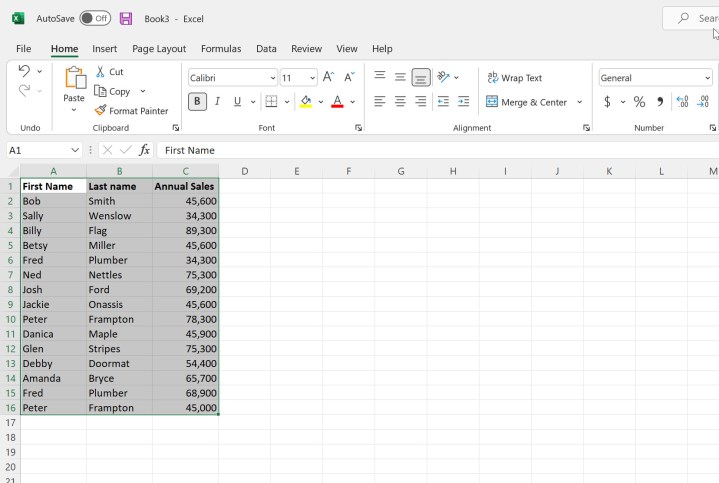
Step 1: Select the portion of your data where you want to locate duplicates. In our example, we’re selecting our entire table. Note that conditional formatting won’t work if you are using pivot tables in Microsoft Excel.
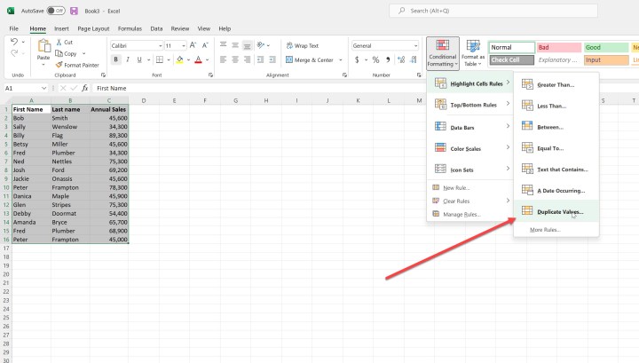
Step 2: Select Conditional Formatting from the Home menu, then choose Highlight Cell Rules > Duplicate Values…
Step 3: You’ll be presented with a dialog that lets you select whether to show duplicate or unique values (we want the former, of course) and how you want the data highlighted. You can choose from the drop-down list or create a custom format.
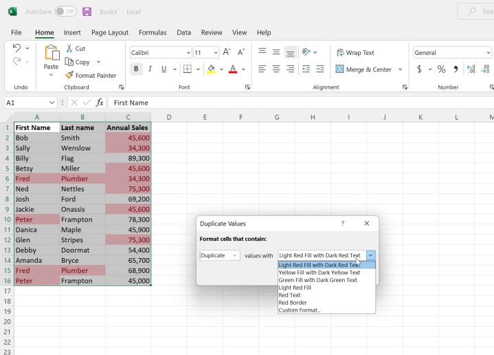
Step 4: Once you’ve selected an option or clicked OK, your duplicate data will be highlighted. This can be textual or numeric data, and it can include any number of columns.

Using the Remove Duplicates function
You can also elect to have Excel remove any duplicate data from your spreadsheet. Use this function with caution – it’s probably a good idea to back up your spreadsheet first.
Step 1: First, select the columns where you want to remove duplicates. Here, we’re selecting the entire table. Note that Remove Duplicates will only remove those items where the values are identical across rows or from individual cells if a single column is selected.
In our example, the last three rows contain duplicate data.

Step 2: Select the Data menu, then click Remove Duplicates. In the dialog box that pops up, you’ll be presented with several options. First, you can identify if your data has headers. Second, you can choose which columns to include or exclude.
When you’re ready, click OK.
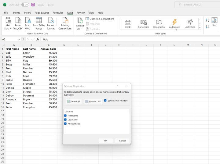
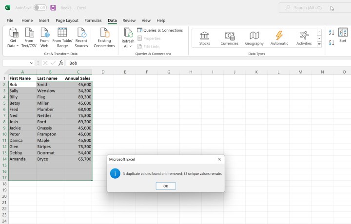
Step 3: You’ll be presented with a dialog that will indicate how many duplicate values were found and removed and how many unique values remain. Note that the last three columns in our data were removed.
Note that it is also possible to use VLOOKUP in Excel to find duplicate data.
Getting to grips with these advanced features turns what appears to be a plain grid of numbers into a powerful tool. Want more tricks? Here’s how to use the concatenate function in Excel.


